 |
6.2 Command group IMAGE |
In EMMENU the images are stored as an array of images: IMAGE(1), IMAGE(2), ... The number of images in this array depends on the amount of memory installed in your workstation and the dimension of your CCD chip.
For example: if there is a 2kx2k CCD chip in the camera with a dynamic of 12 bit (=> 16 bit storage needed for one pixel) , then a single image needs 8 mega bytes storage (8 MB = 8388608 bytes).
The IMAGE command group now provides the operations for displaying and scaling the images as well as navigating within the image array and doing some calculations with the images.
|
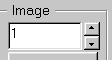
The current image number can be changed either by directly typing the desired image number into the corresponding edit field or by clicking on
the spin control to decrease/increase the current image number. Optionally the image is automatically displayed if the image number has been changed.
Enable/Disable this option in the Display setup dialog.
A click on the button ![]() will display the current image in the next viewport.
will display the current image in the next viewport.
More about the viewport concept in Frequently Asked Questions (FAQ) section GENERAL
A click on the button ![]() will display the current image in the next viewport.
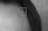
Then the mouse cursor will change and automatically move
to the center of that viewport. You are now in zoom mode. Differently from the
simple grey value analyze tool using the left and right mouse keys over the
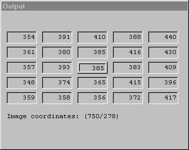
display area the output window ( if open ) changes its layout and displays the
real 16-bit greyvalue data of the pixels under the center of the mouse pointer.
A click on the left button zooms into the image with the clicked pixel as new
center of the zoomed image ( if possible ). A click on the right button zooms
out. You can leave zoom mode pressing any key.
will display the current image in the next viewport.
Then the mouse cursor will change and automatically move
to the center of that viewport. You are now in zoom mode. Differently from the
simple grey value analyze tool using the left and right mouse keys over the
display area the output window ( if open ) changes its layout and displays the
real 16-bit greyvalue data of the pixels under the center of the mouse pointer.
A click on the left button zooms into the image with the clicked pixel as new
center of the zoomed image ( if possible ). A click on the right button zooms
out. You can leave zoom mode pressing any key.
 |
 |
The 'User data' dialog is activated with ![]()
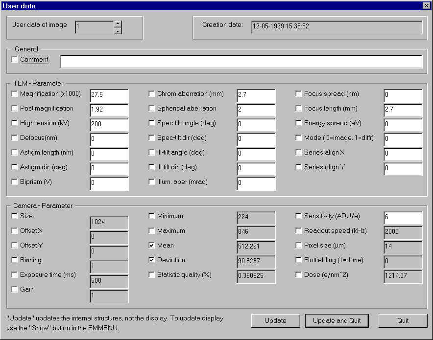 |
This dialog shows the user data of the corresponding image. There are 5 groups for different purposes. In the upper left corner is the corresponding image number displayed. An other image is selected if you change this number.
In the upper right corner the acquisition date and time of the current image are shown. These values are unchangeable.
The next three sections are 'General', 'TEM-Parameter' and 'Camera-Parameter'. Each of the particular items has a little checkbox indicating that this item is also displayed in the image (in the overlay level on the screen).
The maximum of selectable items is 10. In the dialog above Mean and Deviation will be displayed together with the image data.
In the 'General' group is an edit field where you can enter a comment up to 79 characters.
Both other groups, 'TEM-Parameter' and 'Camera-Parameter' show the data of the TEM and CCD camera. You can changed the data in the fields with the white background.
Use ![]() to enter the 'Scaling' dialog. There are five index cards each for the settings of a different display mode.
to enter the 'Scaling' dialog. There are five index cards each for the settings of a different display mode.
Scaling in real space:
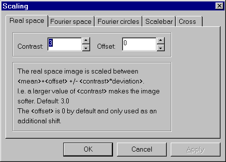 |
EMMENU displays the real space images using the so-called Mean-Deviation method. The mean value and the root mean square deviation are computed and the values Low and High are defined by Low := Mean + Offset - Contrast * Deviation High := Mean + Offset + Contrast * Deviation All pixel values out of the range [Low..High] are clipped to Low or High, respectively, if necessary. Then the ( possible clipped ) values are rescaled to [0..255] and displayed. Note: Only the displayed data is scaled. The image holds still its original data. See also examples at the end of this chapter. |
Scaling in Fourier space:
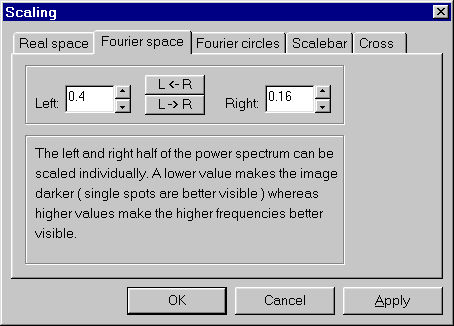 |
In EMMENU the left and the right side of the power spectrum might be scaled differently. This enhances the interpretation.
The numbers are scale factors that are multiplied to the power spectrum data. It is difficult to suggest "good" scaling
factors, since this is very image dependent. Use the L->R to copy the value of the left edit field into the right one. Analogous use R->L to transfer the value of the right edit field into the left one See also examples at the end of this chapter. |
Circles in Fourier space:
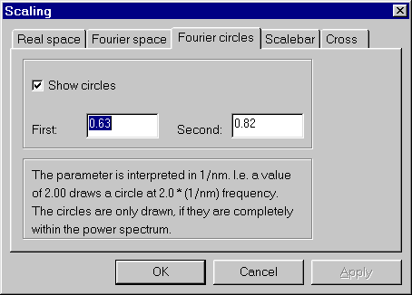 |
EMMENU offers the possibility to display 2 circles at user defined frequences. To display those 2 circles, check the option
Show circles and enter the desired values in the edit fields. Those 2 circles are red. Note: The circles are only displayed, if they fit completely into the power spectrum. See also examples at the end of this chapter. |
Scalebar:
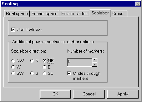 |
EMMENU offers a scalebar option. This option applies both to images in real space and to power spectra. To switch the scalebar
option on or off, check or uncheck the box labeled Use scalebar. In real space a horizontal bar and its length are displayed in the upper right corner of the image. In the power spectrum the scalebar is displayed as a line beginning in the center and pointing into one of the 8 possible directions. The scalebar has a user specified number of markers showing the corresponding frequencies. Additionally it is possible to show circles through the markers. To distinguish those circles from the 2 (red) user defined circles, those circles are green. |
Scaling of crosscorrelation images:
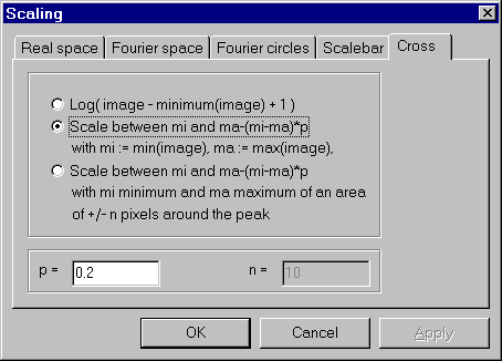 |
The scaling of cross correlations for display purposes is always a little bit tricky. The default values as shown in the
dialog to the left are "good" settings coming from experience. Nevertheless there are sometimes images whose displayed
correlations are just completely black or completely white or anyway unusable. There are 3 possibilities of scaling available as described right to the radio buttons. Select one of those and play with the parameters p and n to receive good display results. ( Sorry, there is no general rule available. ) Note:This dialog influences ONLY how the correlation data are displayed. The peak search ( with subpixel accuracy ) is performed on the original data. |
Scaling examples:
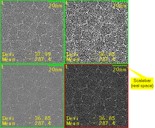 |
This example shows the influence of the parameters Contrast and Offset in the register card Real space.
|
||||||||||||
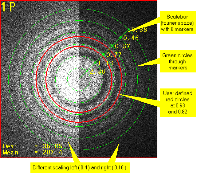 |
This example shows the scaling possibilities in the fourier space. The left side of the spectrum is scaled with 0.4 and the right side with 0.16 in the Fourier space register card. Note that the left side is much brighter. The red circles are set to the corresponding frequencies 0.63 ( outer red circle ) and 0.82 ( inner red circle ) in the Fourier circles register card. In the register card Scalebar the scalebar is enabled, the direction is set to NorthEast(NE), corresponding with up-right, 6 markers are selected and the option Circles through markers is checked. |
A click on ![]() opens the 'Arithmetic' dialog, where you can do some image calculations.
opens the 'Arithmetic' dialog, where you can do some image calculations.
 |
This page is divided in three sections. In the upper section you can select the destination image A ( = result of the arithmetic operation), the source images B and C and the constant floating point value D. Some of the operations do not need B, C or D. In this case the current values for these parameters are simply ignored.
In the middle 'Operations' section you can select one of the listed, predefined operations.
| A := D | Fill image A with constant value nearest_integer(D) | A := LN(B*D) | Multiply image B with constant value D and calculate the natural logarithm of B*D. The nearest integer of the result is stored into destination image A. Note: B*D must be greater than 0 ! |
| A := B + D | Add the integer value nearest_integer(D) to image B, then store the result into image A | A := Rotate90(B, D) | Rotate image B counter-clockwise by 90 degrees and store the result into destination image A |
| A := B * D | Multiply image B with constant value D and copy the result into destination image A | A := MirrorX(B) | Mirror image B at horizontal axis and store the result into destination image A |
| A := B * D + C | Multiply image B with constant value D then add image C and store the result into destination image A | A := MirrorY(B) | Mirror image B at vertical axis and store the result into destination image A |
| A := B * D - C | Multiply image B with constant value D then subtract image C and store the result into destination image A | A := WrapX(B, D) | Wrap the image n pixels to the right. Pixels shifted out of the image are shifted into the image from left. The result is stored into image A. n = nearest_integer( D ). Negative D means shift to the left |
| A := B * D * C | Multiply image B with constant value D and image C then store the result into destination image A | A := WrapY(B, D) | Wrap the image n pixels up. Pixels shifted out of the image are shifted into the image from down. The result is stored into image A. n = nearest_integer(D). Negative D means shift downwards. |
| A := (B*D) / C | Multiply image B with constant value D then divide by image C and store the result into destination image A. Watch out for division by zero ! | A := LocalScale(B,D) | Rescale the image by computing the locale minimum and maximum in a D*D environment (D odd). Scale the current value relative to those locale minima and maxima. |
| A := ABS(B*D) | Multiply image B with constant value D then calculate the absolute value and store the result into destination image A | A := CircMask(B,D) | Create a circular exponential mask, multiply it to image b and store the result in image A, with b := B-Mean(B). The size of the mask is determined by D, which specifies the size in percent of the radius, i.e. 1.0 means full and .5 means half radius |
| A := ABS(B*D+C) | Multiply image B with constant value D and add image C then calculate the absolute value and store the result into destination image A | A := Testpattern(D) | Create a testpattern into image A, depending on D: D=0: Chess board, D=1: Quadratic shading, D=2: linear shading, D=3: Circles, D=4: Dots, D=5: Horizontal lines and D=6: Vertical lines |
| A := ABS(B*D-C) | Multiply image B with constant value D and subtract image C then calculate the absolute value and store the result into destination image A | A := Touch | This command makes an image valid, even if there is no data in it coming from either exposure, file I/O or other arithmetic operation. Note: This command is for experienced users only. |
Example 1: the current selected operation is "A := ABS( B*D + C )", destination image is 2, source image B is 3 and source image C is 4 and the constant value D is 1.3. Then image 3 is internally multiplied by 1.3 and (since all images are of data type SHORT = signed 16 bit integer) the result of the multiplication is converted to SHORT type. After that, image 4 is added to the intermediate result and finally the absolute value is computed and stored into image 2. The images B and C (here images 3 and 4) are not changed.
Example 2: The current selected operation is "A := D", destination image is 2, source image B is 3 and source image C is 4 and the constant value D is 1.3. Then image 2 is set to 1 (since the nearest integer of 1.3 is 1). The image numbers of image B and C are ignored.
Last update: